Montek Singh Gill

In this post, we shall illustrate the intuitive meaning of the Laplacian of a multivariable function as a measure of the concavity of the graph of the function, where this concavity is itself measured via average values in local neighbourhoods.

The Laplacian

Let $f \colon \mathbb{R}^d \to \mathbb{R} \colon (x_1,\dots,x_d) \mapsto f(x_1,\dots,x_d)$ be some smooth¹ multivariable function. To each such $f$ , there is associated it’s Laplacian $\nabla^2f \colon \mathbb{R}^d \to \mathbb{R}$ , defined by

$\nabla^2f := \frac{\partial^2 f}{\partial x_1^2} + \cdots + \frac{\partial^2 f}{\partial x_d^2}.$

The purpose of this note is to illustrate the intuitive meaning of the Laplacian.²

A Hint at the Answer

We note that the Laplacian $\nabla^2f$ is exactly the divergence of the gradient of $f$ . Given a vector field on $\mathbb{R}^d$ and $\mathbf{p} \in \mathbb{R}^d$ , we know that if the vectors at neighbouring points point outward away from $\mathbf{p}$ , than the divergence of the field at $\mathbf{p}$ is positive, whereas if they all point inward toward $\mathbf{p}$ the divergence is positive, and more generally the numerical value of the divergence captures exactly the balance of inward and outward pointing neighbouring vectors.³

**Figure 1.** The divergence at the lefthand point is positive, whereas, at the righthand point, it is negative.

In the case of the gradient of $f$ , what does it mean if neighbouring vectors point outward? Recalling that the gradient points in the direction of steepest ascent (along the graph of $f$ ), we see that in such a case the graph of $f$ at $\mathbf{p}$ must be concave up. Conversely, if the neighbouring vectors point inward, the graph of $f$ at $n\mathbf{p}$ must be concave down.

**Figure 2.** At local minima, the divergence of the gradient is positive, whereas, at local maxima, it is negative.

This leads us to think that $(\nabla^2f)(\mathbf{p})$ is a measure of the concavity of the graph of $f$ at $\mathbf{p}$ . In fact, when $n = 1$ , $\nabla^2f$ is just the ordinary second derivative, and it is of course well-known that the ordinary second derivative is a measure of the concavity of the graph. Thus we suspect that, in this particular sense, the Laplacian is the natural extension of the ordinary second derivative of single variable functions to multivariable functions.

Measuring Concavity Via Average Values

Consider the ordinary second derivative of a single variable function. In what sense exactly is this second derivative a measure of the concavity of the graph of the function? As it is the rate of change of the first derivative, using the interpretation of the first derivative as the slope of the graph, it is clear that a positive second derivative means upward concavity and a negative second derivative means downward concavity. Moreover, the rate of change of the slope clearly correlates with the degree of concavity.

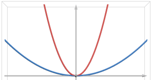
**Figure 3.** Along both the red and blue curves, as one passes the origin from left to right, the slope changes from negative to positive. Thus, at the origin, the second derivative is positive in both cases. However, the incremental change in the slope per change in the abscissa is clearly larger in the case of the red curve, and so the second derivative is larger in the case of the red curve. In this way, the second derivative is a measure of the degree of concavity at the origin.

In place of the rate of change of the slope, we can measure the degree of the concavity in a different way, by looking at local average values. At a given point $p$ , consider the values of the function at neighbouring points. Certainly, in the case of upward concavity, neighbouring values are larger than $f(p)$ , the value at $p$ , and, in the case of downward concavity, the neighbouring values are lower than $f(p)$ . Moreover, for sufficiently small neighbourhoods, in the case of upward concavity, the degree of concavity correlates with the rate at which the average neighbouring value rises above $f(p)$ with the size of the neighbourhood (and a similar statement holds for downward concavity). In the case of mixed concavity, such as saddle points, there is a mixture of neighbouring values above and below $f(p)$ , and these make opposing contributions to the average deviation from $f(p)$ . We are thus led to consider average values in local neighbourhoods of $p$ .

Let us consider an example.

**Figure 3.** As the radius of the circle increases, the concavity at the origin decreases.

In Figure 3 are depicted the circles described by $x^2 + (y-R)^2 = R^2$ for various values of $R$ . One can see that, as $R$ increases, the concavity at the origin decreases. Moreover, a simple calculation shows that $\frac{d^2y}{dx^2}\vert_{x=0} = \frac{1}{R}$ . Thus the second derivative, the one-dimensional Laplacian, is proportional to the concavity. Next, consider the values at the neighbouring points $-r$ and $r$ , for small $r$ , and form their average; this average is $R - \sqrt{R^2-r^2}$ . We are interested in how this average behaves as $r$ changes. Near zero, we have that

$\begin{aligned} R - \sqrt{R^2-r^2} &= R - R\sqrt{1-\frac{r^2}{R^2}} \\ &= R - R\left(1 - \frac{1}{2}\frac{a^2}{R^2} + \cdots\right) \\ &\approx \frac{1}{2R}r^2. \end{aligned}$

Thus, we see that, in sufficiently small neighbourhoods, the rate at which the average value rises with $r$ is (up to the constant $\frac{1}{2}$ ) exactly the value $\frac{1}{R}$ of the Laplacian.

We can generalize the analysis in the above example as follows. For an arbitrary smooth function $f \colon \mathbb{R} \to \mathbb{R}$ and a point $p \in \mathbb{R}$ , consider the average of the two values at $p-r$ and $p+r$ . This average is given by

$\mathrm{A}_p^{\mathrm{S}}(r) := \frac{f(p-r) + f(p+r)}{2}.$

This is clearly smooth in $r$ , and, moreover, easy calculations demonstrate that

$\begin{aligned} \mathrm{A}_p^{\mathrm{S}}(0) &= f(p) \\ (\mathrm{A}_p^{\mathrm{S}})'(0) &= 0 \\ (\mathrm{A}_p^{\mathrm{S}})''(0) &= f''(p). \end{aligned}$

Thus, by Taylor’s expansion, we have that

$\mathrm{A}_p^{\mathrm{S}}(r) = f(p) + \left[\frac{1}{2}f''(p)\right]r^2 + o(r^2).$

This yields an interpretation of the Laplacian as a measure of the rate at which the average value deviates from $f(p)$ as we expand the region over which the average is taken. This is a specific sense in which the second derivative, the one-dimensional Laplacian, captures the concavity of the graph.

In the above analysis, we considered averages of values at points near $p$ . Specifically, we considered the average of the values on the set $\{p-r,p+r\}$ . This is the zero-dimensional spherical boundary of the neighbouring interval $[p-r,p+r]$ , a one-dimensional ball, and it is just as natural, if not more natural, to consider the average instead over this interval. At $p$ , the average value of $f$ on $[p-r,p+r]$ is

$\mathrm{A}_p^{\mathrm{B}}(r) := \frac{1}{2r}\int_{p-r}^{p+r}f(x)\,dx.$

Our goal here is to demonstrate a connection between these average values $\mathrm{A}_p^{\mathrm{B}}(r)$ and the Laplacian $(\nabla^2f)(p) = f''(p)$ . As before, we thus investigate the local behaviour of $\mathrm{A}_p^{\mathrm{B}}$ at $r = 0$ . At $r = 0$ , the above expression is ill-defined and instead the average value $\mathrm{A}_p^{\mathrm{B}}(0)$ is of course set to be $f(p)$ ; an easy application of L’Hopital’s rule shows that $\mathrm{A}^{\mathrm{B}}_p$ is then continuous. In fact, we can show that $\mathrm{A}_p^{\mathrm{B}}$ is smooth (this is non-obvious only at $r=0$ ). To see this, set $G(r) := \int_{p-r}^{p+r}f(x)\,dx$ . By the fundamental theorem of calculus, $G$ is smooth. For any $k \ge 1$ , by Taylor’s theorem, using the integral form of the remainder, we have that

$G(r) = G(0) + G'(0)r + \frac{G''(0)}{2!}r^2 + \cdots + \frac{G^{(k)}(0)}{k!}r^k + \int_0^r \frac{G^{(k+1)}(a)}{k!}(r-a)^k\,da.$

We can identify the derivatives of $G$ : first, it is clear that $G(0) = 0$ and, by the fundamental theorem of calculus, $G'(r) = f(p+r) + f(p-r)$ , from which it follows that $G'(0) = 2f(p)$ . In fact, a simple induction shows that $G^{(n)}(0)$ vanishes for even $n$ and $2f^{(n-1)}(p)$ for odd $n$ . Consider the case $k = 1$ . We get that

$G(r) = 2f(p)r + \int_0^r G^{(2)}(a)(r-a)\,da.$

Using the substitution $a = rb$ , we can rewrite the integral remainder term and get

$\int_0^r G^{(2)}(a)(r-a)\,da = r^2\int_0^1 G^{(2)}(rb)(1-b)\,db.$

Now, noting that $\mathrm{A}_p^{\mathrm{B}}(r) = \frac{G(r)}{2r}$ , we find that

$\mathrm{A}_p^{\mathrm{B}}(r) = f(p) + \frac{r}{2}\int_0^1 G^{(2)}(rb)(1-b)\,db.$

The smoothness of $\mathrm{A}_p^{\mathrm{B}}$ now follows from the Leibniz integral rule combined with the fact that $(r,b) \mapsto G^{(2)}(rb)(1-b)$ defines a smooth function on $\mathbb{R}^2$ .

Let us now return to investigating the local behaviour of $\mathrm{A}_p^{\mathrm{B}}$ at $r = 0$ . The above expression can be used to compute $(\mathrm{A}_p^{\mathrm{B}})'(0)$ . However, having established the smoothness of $\mathrm{A}_p^{\mathrm{B}}$ , we can compute this derivative more simply as follows. By the quotient rule and the fundamental theorem of calculus, for non-zero $r$ , we have that

$(\mathrm{A}_p^{\mathrm{B}})'(r) = \frac{rf(p+r) + rf(p-r) - G(r)}{2r^2}.$

Using smoothness of $\mathrm{A}_p^{\mathrm{B}}$ (and the consequent smoothness of $(\mathrm{A}_p^{\mathrm{B}})'$ ), we see that

$\begin{aligned} (\mathrm{A}_p^{\mathrm{B}})'(0) &= \lim_{r \to 0}\frac{rf(p+r) + rf(p-r) - G(r)}{2r^2} \\ &= \lim_{r \to 0}\frac{f(p+r) + rf'(p+r) + f(p-r) - rf'(p-r) - f(p+r) - f(p-r)}{4r} \\ &= \lim_{r \to 0}\frac{f'(p+r) - f'(p-r)}{4} \\ &= 0 \end{aligned}$

where in the second line we have used L’Hopital’s rule. In a similar manner, we can also compute the second derivative $(\mathrm{A}_p^{\mathrm{B}})''(0)$ . For non-zero $r$ , we have that

$(\mathrm{A}_p^{\mathrm{B}})''(r) = \frac{r^2f'(p+r) - r^2f'(p-r) - 2rf(p+r) - 2rf(p-r) + 2G(r)}{2r^3}.$

Using smoothness of $\mathrm{A}_p^{\mathrm{B}}$ , we see that

$\begin{aligned} (\mathrm{A}_p^{\mathrm{B}})''(0) &= \lim_{r \to 0}\frac{r^2f'(p+r) - r^2f'(p-r) - 2rf(p+r) - 2rf(p-r) + 2G(r)}{2r^3} \\ &= \lim_{r \to 0}\frac{r^2f''(p+r) + r^2f''(p-r)}{6r^2} \\ &= \lim_{r \to 0}\frac{f''(p+r) + f''(p-r)}{6} \\ &= \frac{1}{3}f''(p) \end{aligned}$

where, again, in the second line we have used L’Hopital’s rule. The Laplacian of $f$ at $p$ has made an appearance. Using Taylor’s theorem for $\mathrm{A}_p^{\mathrm{B}}$ , we may now write the following local expression

$\mathrm{A}_p^{\mathrm{B}}(r) = f(p) + \left[\frac{1}{6}f''(p)\right]r^2 + o(r^2).$

As suspected, (for sufficiently small neighbourhoods, and up to a constant) the second derivative $f''(p)$ at $p$ controls the rate at which the average value deviates from $f(p)$ as we expand the neighbourhood.

In the case of a one-dimensional domain, we have now considered averages over spheres and balls. There is yet another form of average of nearby values which we can link to the ordinary second derivative, the one-dimensional Laplacian. The ordinary second derivative can be expressed as the limit

$f''(p) = \lim_{r \to 0}\frac{f(p+r) + f(p-r) - 2f(p)}{r^2}.$

(One can easily check that the limit above does indeed coincide with the second derivative using L’Hopital’s rule.) From this, it follows that, as $r \to 0$

$\frac{f(p+r) + f(p-r)}{2} \approx f(p) + \left[\frac{1}{2}f''(p)\right]r^2 + o(r^2).$

This simply recovers the result above in the case of an average over a neighboring sphere. In this case, however, we interpret the lefthand side as the average of neighbouring values along the positive and negative axial directions, and denote by $\mathrm{A}^{\mathrm{X}}_p(r)$ . We do so because we can perform an analogous analysis in higher dimensions. For example, consider the case of two dimensions. In this case, the Laplacian $(\nabla^2f)(\mathbf{p})$ is the sum $f_{xx}(\mathbf{p}) + f_{yy}(\mathbf{p})$ and can be expressed as the limit

$f_{xx}(\mathbf{p}) + f_{yy}(\mathbf{p}) = \lim_{r \to 0}\frac{f(p_1+r,p_2) + f(p_1-r,p_2) + f(p_1,p_2+r) + f(p_1,p_2-r) - 4f(p_1,p_2)}{r^2}.$

(Once again, one can easily check that the limit above does indeed coincide with the Laplacian using L’Hopital’s rule.) From this, it follows that, as $r \to 0$

$\begin{aligned} \mathrm{A}^{\mathrm{X}}_p(r) &:= \frac{f(p_1+r,p_2) + f(p_1-r,p_2) + f(p_1,p_2+r) + f(p_1,p_2-r)}{4} \\ &= f(p) + \left[\frac{1}{4}(\nabla^2f)(p)\right]r^2 + o(r^2). \end{aligned}$

Again, the lefthand side is the average of neighbouring values along the axial directions, and the result tells us that (for sufficiently small distances to $\mathbf{p}$ , and up to a constant) the Laplacian at $p$ controls the rate at which this average value deviates from $f(p)$ as we expand the neighbourhood.

A final remark for this section: note that in every local expression, there was no linear term in $r$ . This makes sense because each averaging function is clearly an even function of $r$ .

The Intuitive Meaning of the Laplacian

In one dimension, the prior section provides a satisfying answer to the question of the intuitive meaning of the Laplacian. In fact, this interpretation holds true in all dimensions. The specific result, for smooth $f \colon \mathbb{R}^d \to \mathbb{R}$ , is that

$\begin{aligned} \mathrm{A}_{\mathbf{p}}^{\mathrm{S}}(r) &= f(\mathbf{p}) + \left[\frac{1}{2d}(\nabla^2f)(\mathbf{p})\right]r^2 + o(r^4) \\ \mathrm{A}_{\mathbf{p}}^{\mathrm{B}}(r) &= f(\mathbf{p}) + \left[\frac{1}{2(d+2)}(\nabla^2f)(\mathbf{p})\right]r^2 + o(r^4) \\ \mathrm{A}_{\mathbf{p}}^{\mathrm{X}}(r) &= f(\mathbf{p}) + \left[\frac{1}{2d}(\nabla^2f)(\mathbf{p})\right]r^2 + o(r^4). \end{aligned}$

For a proof of the first two, see The Laplacian and Mean and Extreme Values by Jeffrey S. Ovall (The American Mathematical Monthly, vol. 123, pp. 287-291 (2016)). As for the third, it follows from the identity

$(\nabla^2f)(\mathbf{p}) = f_{x_1x_1}(\mathbf{p}) + \cdots + f_{x_dx_d}(\mathbf{p}) = \lim_{r \to 0}\frac{\sum_{i=1}^d [f(\mathbf{p} + r\mathbf{e}_i) + f(\mathbf{p} - r\mathbf{e}_i)] - 2df(\mathbf{p})}{r^2}.$

where $\mathbf{e}_1, \dots, \mathbf{e}_d$ denote the standard basis vectors of $\mathbb{R}^d$ . Note that, in the case $d = 1$ , these reduce to the local expressions which we derived in the prior section (except that the remainder term is given the stronger expression $o(r^4)$ instead of $o(r^2)$ ).

In fact, in the same aforementioned paper, higher order approximations are provided, from which one can easily derive the well-known fact that, if, for a given $f$ , the Laplacian $\nabla^2f$ is zero in some open region $\Omega$ , then the value of $f$ at any point in $\Omega$ is exactly equal to average of $f$ over any ball $B$ or the boundary sphere $\partial B$ , where $\overline{B} \subseteq \Omega$ , centred at that point.

The Intuitive Meaning of the Laplace, Poisson, Heat and Wave Equations

We have now completely answered the question of the intuitive meaning of the Laplacian. It is natural now to consider the intuitive meaning of differential equations in which the Laplacian appears. Let us consider the Laplace, Poisson, Heat and Wave equations. We can gain an intuition for these based on the physical contexts in which they arise.

The Laplace and Poisson Equations. Let us begin with the Laplace and Poisson equations. For a scalar field $f \colon \mathbb{R}^d \to \mathbb{R}$ , these are the equations $\nabla^2f = 0$ and $\nabla^2f = \alpha$ , respectively, where $\alpha$ is some specified function. For example, if $\rho$ denotes the mass density in three-dimensional space, the corresponding gravitational potential $\varphi$ satisfies

$\nabla^2\varphi = 4\pi G\rho.$

The corresponding gravitational force is given by $-\nabla\varphi$ , and so a particle is always pushed in the direction of decreasing potential $\varphi$ , with a force magnitude proportional to the rate of decrease; in particular, near any given point in space $\mathbf{p}$ , a particle is pushed toward or away from $\mathbf{p}$ depending on whether or not this increases or decreases $\varphi$ . Here, whether or not there is an increase or decrease can be assessed by measuring the deviation of the average of the nearby values from the potential $\varphi(\mathbf{p})$ at $\mathbf{p}$ , which, as we have seen, is exactly what is measured by the value of the Laplacian $(\nabla^2\varphi)(\mathbf{p})$ . The above equation says that the Laplacian is proportional to the mass density, and so it says that particles are pulled toward regions of positive mass density, with a force magnitude which is proportional to the mass in the region.

In the case where the mass density $\rho$ is identically zero, the potential $\varphi$ satisfies Laplace’s equation $\nabla^2\varphi = 0$ . This equation says that, at any point $\mathbf{p}$ , the value of the potential at $\mathbf{p}$ is exactly equal to the average of the neighbouring values. Thus, at any point $\mathbf{p}$ , a particle is not compelled to move in any direction (it is in an equilibrium state), and we get a zero gravitational field, as expected from the zero mass density. \\
One can make very similar interpretations for the equation $\nabla^2V = -\frac{1}{\varepsilon_0}\rho$ for the electrostatic potential $V$ .

The Heat Equation. Next, let us consider the heat equation. This is the equation

$\frac{\partial u}{\partial t} = \alpha\left(\frac{\partial^2 u}{\partial x_1^2} + \cdots \frac{\partial^2 u}{\partial x_d^2}\right)$

where $u \colon \mathbb{R}^d \times \mathbb{R} \to \mathbb{R}$ represents temperature at a given point at a given time and $\alpha$ is some non-negative constant. At a given time $t_0$ , the righthand side may be written as $\alpha\nabla^2u(t_0, -)$ . The equation determines the evolution of the temperature throughout space over time, which is to say the flow or diffusion of heat throughout space. At any given time $t_0$ , and spatial point $\mathbf{p}$ , the value of $\nabla^2u(t_0, -)$ at $\mathbf{p}$ represents the deviation of the average of the neighbouring temperature values from the temperature at $\mathbf{p}$ at time $t_0$ . Thus, the equation says that the rate of change of the temperature at $\mathbf{p}$ at $t_0$ is proportional to this difference between surrounding temperatures and the temperature at $\mathbf{p}$ . This is intuitive and aligns with Newton’s law of cooling. The non-negative constant $\alpha$ then represents the ease with which heat flows through the medium and so is referred to as the thermal diffusivity of the medium.

The Wave Equation. Finally, let us consider the wave equation. This is the equation

$\frac{\partial^2 u}{\partial t^2} = v^2\left(\frac{\partial^2 u}{\partial x_1^2} + \cdots \frac{\partial^2 u}{\partial x_d^2}\right)$

where $u \colon \mathbb{R}^d \times \mathbb{R} \to \mathbb{R}$ represents the size of a wave disturbance at a given point at a given time and $v$ is a non-negative constant. At a given time $t_0$ , the righthand side may be written as $v^2\nabla^2u(t_0, -)$ . The equation determines the propagation of the wave throughout space over time. At any given time $t_0$ , and spatial point $\mathbf{p}$ , the value of $\nabla^2u(t_0, -)$ at $\mathbf{p}$ represents the deviation of the average of the neighbouring disturbances from the disturbance at $\mathbf{p}$ at time $t_0$ . Thus, the equation says that the acceleration of the point $\mathbf{p}$ , due to the wave, is proportional to the difference between the surrounding disturbances and the disturbance at $\mathbf{p}$ . This is similar to simple harmonic motion where the acceleration of a particle is proportional to its distance from an equilibrium point, except that here the equilibrium is the current state of the $\mathbf{p}$ and the acceleration takes into account the disturbance not only at $\mathbf{p}$ but at points nearby $\mathbf{p}$ . The non-negative constant $v$ then represents the ease with which the disturbances at points nearby to $\mathbf{p}$ impact the disturbance at $\mathbf{p}$ itself, from which it is not too difficult to guess that $v$ turns out to correspond to the speed of the wave.

We can consider the Laplacian, and all other related material here, for, e.g., $\mathrm{C}^2$ functions. For the purposes of this note, however, the degree of smoothness is a distraction, and so we consider only smooth, that is, $\mathrm{C}^\infty$ , functions. ↩︎
The Laplacian, and all other related material here, can of course be considered for functions which are defined only on subsets of $\mathbb{R}^d$. The considerations carry over easily, and so domain considerations are a distraction, and so we restrict to functions defined on all of $\mathbb{R}^d$. ↩︎
Throughout, vectors will be denoted in boldface. ↩︎